VELO testbeam analysis
C. ACDC3 results
C1. Foreword
This page contains
preliminary ACDC3 results. Final results/conclusions will be presented in a dedicated LHCb note.
C2. Principle of the study
Alignment has been performed right after data taking, whenever necessary (new cable configuration or experimental setup movement). All the different situations are summarized on figure 1:
1. ACDC3 Happy Pion Configurations.
One specific
alignment.xml has been produced for each situation, thus leading to 9 possibilities. However, only 4 files are included within the main
VeloACDC package, one for each configuration:
Except for HP3, where reprocessing is necessary to get the alignment of the angled tracks, those files were chosen because they could be used with most of the available dataset. However, other alignment files are available on request to
me. You could also, if you have some time, produce them yourself using the alignment software, an
HowTo page is available.
Next parts present a chronological description of the alignment results. The most up-to-date results are thus at the bottom of this page, but you could read the rest if you want the full story.
C3. A first look
As previously stated, the alignment was performed was performed during the testbeam, as soon as enough statistics were collected (~200000 events). The alignment process, from data collection to xml file production, took few minutes. Once the correct xml file was produced, results with and without alignment could be compared using few macros available
here.
The following plots were obtained for configuration 4, with beam on targets. The first parameters we could compare are the spacepoints residuals, before and after alignment. These are shown on figures 2 and 3:

2. HP4: spacepoints residuals (X coordinate).
|
|

3. HP4: spacepoints residuals (Y coordinate).
|
These figures show a clear improvement of the residuals by the alignment, thus confirming, on 6 modules this time, the encouraging results obtained for 3 modules during the ACDC2 campaign.
A clear improvement was also observed for the vertex reconstruction, which has been tested for the first time during ACDC3 (see
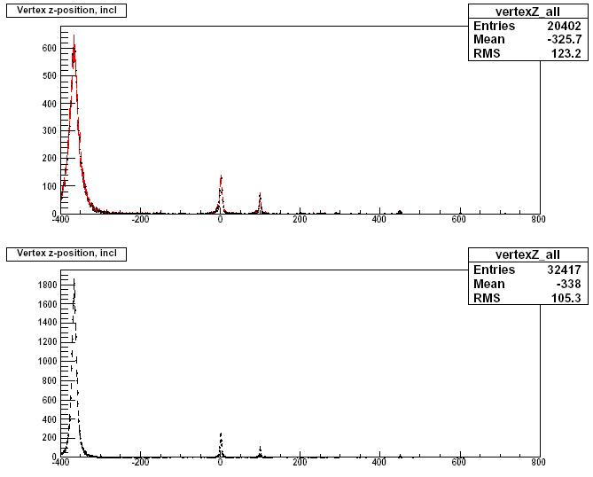
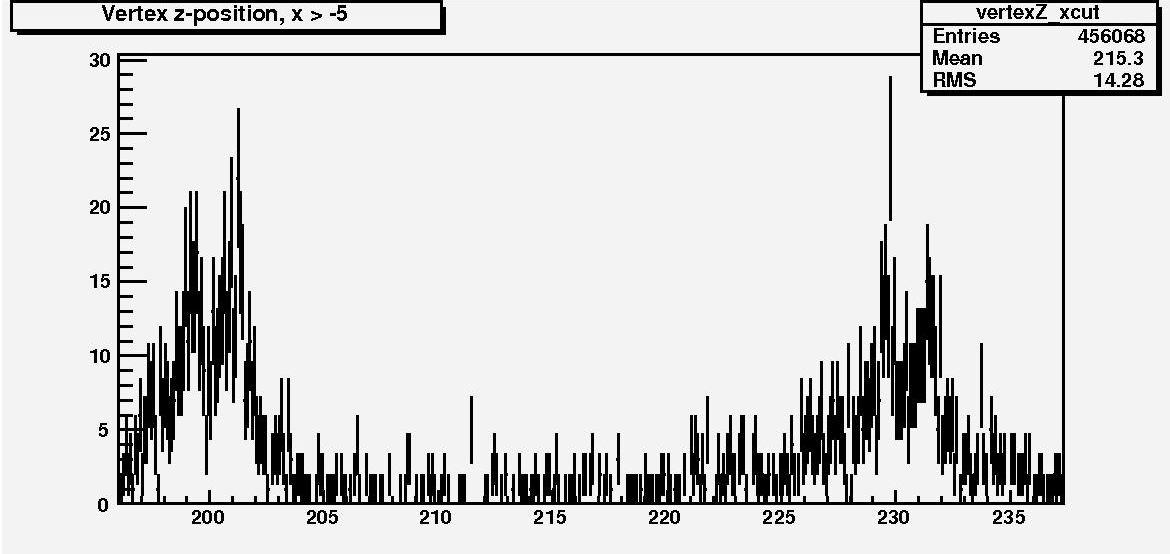
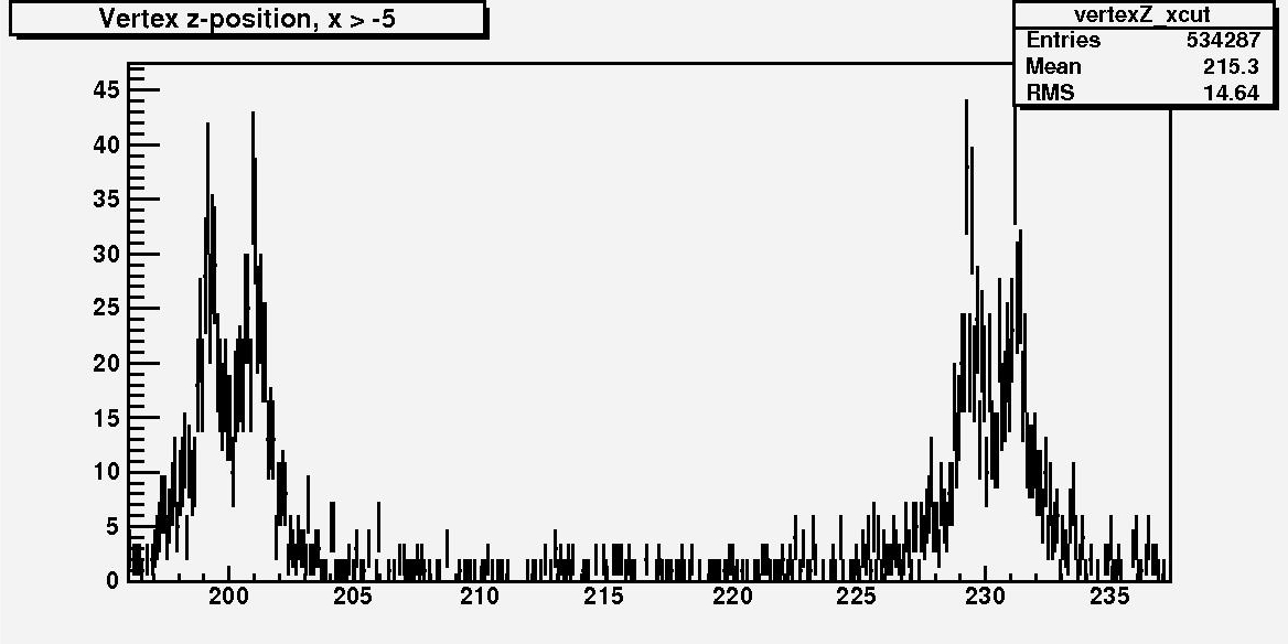
Aras' talk for more details about that). Figure 4 shows the results obtained with and without alignment, running on the main HP4 dataset: 3.7 millions of events.

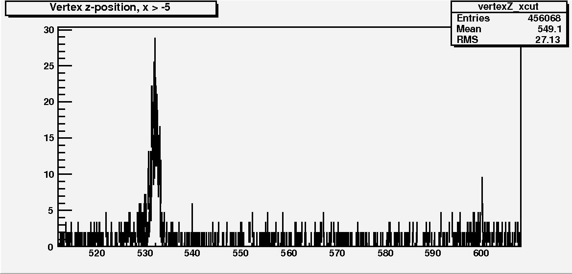
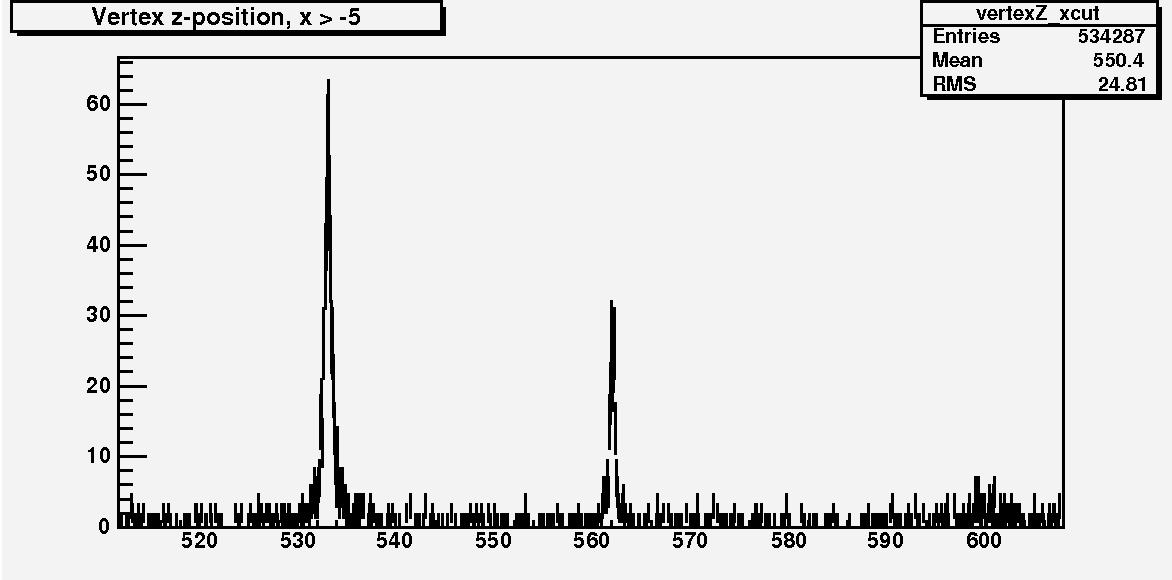
4. Vertices before (top) and after (bottom) alignment.
This figure shows a slight improvment of the number of reconstructed vertices, in particular in the beam window (largest peak). Quantitatively, the numbers of reconstructed vertices in the different targets were:
1. Without Alignment:
- Beam Window : 18456
- Target1 : 1117
- Target2 : 409
2. With Alignment:
- Beam Window : 30229 (+64%)
- Target1 : 1408 (+26%)
- Target2 : 452 (+10%)
From this one could conclude that alignment is providing a good correction of the geometry, at least at first order (ie to ensure a good quality data-taking). Then we went further and looked more closely at the alignment constants which were found.
C4. When alignment is useful: an example
An other important point of ACDC3 alignment was to study the change of the alignment with or without vacuum. To this end, two identical datasets were taken with HP1: one with normal pressure and the other in vacuum (see fig.1). Alignment constants in both situation were compared, thus resulting in figure 5:

5. Misalignment constants in air (open circles) and in vacuum (red dots).
There are one good thing and one bad thing coming out of this plot.
The good point is that alignment is more or less the same with or without vacuum. Largest displacements are of order of 10 microns, which is relatively small. However, as we are only studying one half, this test gave us only information on modules movements w.r.t. each other when going to vacuum. We don't learn anything about boxes movements here. But seeing that modules positions are stable is already a good thing.
The bad point was concerning the alignment constants, in particular rotations around Z axis. A quick look showed that those values were very large (~6 mrad !!!). This was not expected at all. However, another look showed us a periodicity between upstream (values around 6 mrad) and downstream (values around -6 mrad) sensors. This periodicity was eventually tracked down to a bug in the geometry description (phi origin of the phi sensors strips). Once this bug was corrected, we obtained the constants shown on figure 6.

6. Misalignment constants in air (open circles) and in vacuum (red dots) after geometry correction.
X and Y constants were, as expected, unchanged, and Z rotation parameters were more in agreement with what was expected in first place. It should be noted that
this bug would have been very difficult to spot without real data or with a larger setup, this is the perfect example of ACDC3 utility.
C5. Results after correction
Of course, in terms of alignment, this correction was annoying: residual plots are now looking less impressive...
More seriously, the alignment job were all reprocessed with the new geometry, and effect of the correction were significant. For example the figures 7 & 8 shows the spacepoints residuals after correction.

2. HP4: new spacepoints residuals (X coordinate).
|
|

3. HP4: new spacepoints residuals (Y coordinate).
|
It's clear, from these figures, that the residuals before alignment are already quite good, which means that the mechanical alignment of the module is very good. Now we still clearly see the effect of alignment.
C6. Including sensors misalignments into the game.
Sensors misalignments are clearly affecting the residuals distributions. A simple look at Phi residuals as a function of Phi angle proves that easily.

4. HP1: Phi residuals as a function of the Phi angle.
|
|

5. HP2: Phi residuals as a function of the Phi angle.
|
|

6. HP4: Phi residuals as a function of the Phi angle.
|
Banana-shaped residuals are typical effect of misalignments between R and Phi sensors (see
Marco's talk during June 2007 LHCb week to learn more about that).
A method is currently developped in order to solve this problem using tracks, but for the moment the only available information is given by CERN metrology. Putting those measurements into the geometry description, one ends up with the following distribution after alignment:

4. HP1: Phi residuals as a function of the Phi angle.
|
|

5. HP2: Phi residuals as a function of the Phi angle.
|
|

6. HP4: Phi residuals as a function of the Phi angle.
|
Bananas amplitudes are clearly reduced, and one even could expect a large reduction when including results from our fitting method. In any case, this result show that CERN metrology provides a coherent input for the alignment.
C7. Current status and conclusions
The alignment work on ACDC data is now more or less completed. Reprocessed data of HP1/2/3 configurations have been processed, new alignment files were produced and are now included in the head revision of VeloACDC package.
To conclude we present some nice results from the alignment, among others:

7. Comparison of the alignment constants obtained for HP2 and HP4 configurations. For X translations (top), Y translations (middle), and Z rotations (bottom).
|

8. HP4: Inner target run without alignment (zoom on target 3 and 4). Only target 3 is visible.
|
|

9. Inner target run without alignment (zoom on target 3 and 4). Target 4 appears...
|
|

10. HP4: Inner target run without alignment (zoom on modules 23 and 31).
|
|

11. Inner target run without alignment (zoom on modules 23 and 31). The R and Phi sensors peaks are clearly better defined and higher.
|
|
Looking at all these results, we could conclude that:
1. The modules alignment is working as expected, and it's effect on VELO tracking and vertexing is visible.
2. Initial mechanical alignment of the modules is good.
3. Modules are not moving largely when going from air to vacuum (less than 10 micrometers).
4. Including sensor misalignment information slightly improves the residuals.
5. Constants found for different configurations are coherent between each other.
C8. Some more results, including crosstalk correction
A collection of few plots, presenting results obtained for residuals after correcting the crosstalk (see explanations in the following talks :
VELO 310707 and
VELO 240807). The page is accessible
here
A further overview of R-sensor cross-talk has been given at the
VELO workshop in December 2007.
C9. The VELO sensor resolution
The VELO sensor resolution has been studied mainly with HP4 data using tracks of perpendicular incidence.
To be more precise, the tracks have been selected to match the slope of the centre of the beam to ensure minimal multiple scattering, thus selecting very small but not necessarily zero angles.
The resolution has been determined as the sigma of a gaussian fit to the distribution of residuals for a given region in pitch.
The small angle of the tracks (less than 2 mrad) means that their hits all lie in the same pitch region with negligible effects at the border of two pitch regions.
The residuals are calculated as the difference between the hit on a sensor and the extrapolated state given by an unbiased linear track fit (a fit excluding the sensor under study).
To obtain the resolution one has to correct for the extrapolation error of the track fit which contributes to the measurement.
Under the assumption that all sensors have equal performance and that all track hits are in the same pitch region, i.e. all hits should have the same hit resolution, one can compute the relative contribution of the extrapolation error to the residuals (see also
LHCb-2000-099).
The thus obtained correction factors can be applied to the fitted resolutions.
The HP4 data sample is excellent for studying resolutions as it has a closely packed set of sensors, thus avoiding long extrapolations.
The resolutions have been studied with two different data samples from a run with a wide beam and from an inner target run.
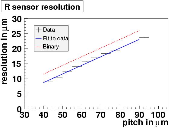
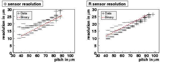
Both lead to consitstent results showing a resolution of roughly 9 microns for a 40 micron pitch, which is significantly better than the resolution expected for a binary readout, thus confirming the VELO readout design choice.
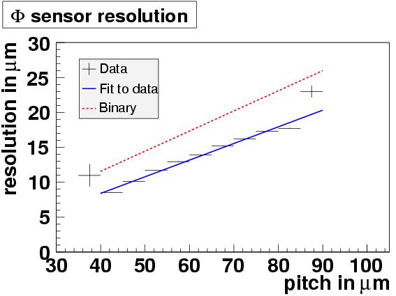
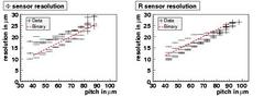
Figures 12 and 13 show the VELO sensor resolution averaged over 6 R and Phi sensors, respectively.
Higher values for very small and very large pitch regions are due to very limited statistics in these regions and should be ignored.
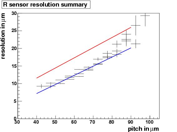
12. R sensor resolution averaged over 6 sensors from HP4.
|
|
13. Phi sensor resolution averaged over 6 sensors from HP4.
|
|
For studying angled tracks a dataset taken in the HP3 configuration has been used.
Here, the beam had an angle of 4 degrees with respect to the normal on the sensor plane.
This means that in the given configuration only four out of the six modules that were read out had a significant number of hits.
Furthermore, the other two modules were located far away from the group of four and thus the extrapolation errors would dominate the measurements.
Unfortunately, one out of the four modules (software number 25, i.e. M29) was very noisy and had to be excluded from the analysis, thus leaving software number 27, 29, and 31.
This, together with the angle of the beam, means that at most two modules contribute to the resolution measurement in a given pitch region.
Also, due to limited statistics only the measurements between a pitch of 50 microns and 70 microns can be trusted.
To be able to apply the correction for the extrapolation error, the track fit had to be restricted to an R-Z-fit only, i.e. only using the R sensor information, because the variation of the strip pitch with radius is different for R and Phi sensors.
Figure 14 shows the resolution of the R sensors for 4 degree tracks.
With the limited amount of data available, the only possible conclusion is that the resolution has improved compared to tracks of perpendicular incidence, as expected.
14. R sensor resolution with tracks of 4 degree incidence.
|
The resolutions obtained here are about 1 micron worse compared to the expectation from Monte-Carlo studies.
An imprioovement is expected from eta corrections, i.e. taking into account the non-linearity of charge sharing with respect to the inter-strip-position of hits.
However, this study already confirms the excellent and coherent performance of all VELO sensors analysed here.
Finally, an interesting study is also the resolution performance without using any misalignment or metrology information.
This shows the raw performance of the modules due to the precision of the assembly.
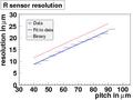
As can be seen in figure 15, the resolution is deteriorated significantly.
However, it is much worse for Phi sensors than for R sensors.
This can be understood as the assembly process was such that the R sensor was placed with a higher precision, which is motivated by the R-Z-tracking in the trigger being based on R sensor information only.
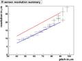
15. R and Phi sensor resolution averaged over 6 sensors, respectively, from HP4 without metrology or alignment corecction.
|
C10. "Still-to-do" list
The points which are still under investigation are:
1. (Optional) How to get alignment constants for more than 6 modules (ie mix 2 configurations in one single job) ?
To be continued...