Existing Alignment Techniques
1. Introduction
This short review only concerns alignment methods based on track parameters
measurements. Indeed other methods, like interferometry, could be used. But in
the VELO context (sensors in vacuum vessel,...) such methods are not applicable,
and alignment by tracks is the most practical option.
The main goal of alignment is to determine the real position of the subdetectors,
in order to take into account this movements in the reconstruction code. Otherwise
this one will assume that the subdetectors are in perfect positions, and then will
not correctly estimate track parameters.
1. The alignment problem
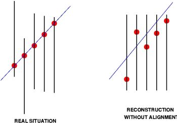
The two part of Fig.1 illustrate the problem. We are here in a very simple case,
with just one misalignment.
What happens in reality is described on the left figure. The particle (blue line)
passing trough the real detector lets its signature: hits (red circles).
The hits are collected and used by the reconstruction code in order to reconstruct
the track. If the alignment is not corrected, the reconstruction code will see the
right figure, ie non-aligned hits. It will then reconstruct a bad quality track, or
even no track at all if the misalignments are very large.
In any case, track parameters will be seriously affected. That's why alignment is mandatory.
2. Minimising the residuals
If we look again at the right figure, we see that the distances between the red circles
and the fitted track (blue line), are larger than on the left figure. These distances
are the residuals, and a good way to align our detector is to minimize them.
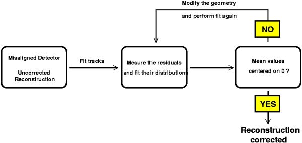
The first idea is to fit a large number of tracks, and to plot the residuals for each
subdetector (in the previous case for the five plates). The mean value of each residual
distribution should then be centered on the misalignment value. We just have to correct
the subdetector coordinates from this value, fit the track again, plot the residuals,...
And so on until the residuals central values are stabilized at 0.
This method could be summarized with the following schedule:
2. Iterative alignment
Of course, in a normal case, there is more than one misaligned parameter, and
residuals are a complex combination of the different misalignment sources. But if
you modelize carefully this sources you would align your detector with a relatively
good accuracy.
However, this method has some drawbacks. The principal problem is that it is iterative,
and iterations are based on biased track fit results (fit with misaligned detector).
Then, even if the method converges, it could leads to biased misalignment values
(offsets to real values).
The solution is to
avoid iterations, in order to avoid biasing the
track fit. That means doing only few times the track fit. However nothing prevents
us to fit the residuals once we have computed them. Non iteratives methods tends to
go into this direction. That's the main subject of the next part.
3. Alignment in one step: fitting the residuals
When you fit a track in a misaligned environment, you had to consider two
different types of fitted parameters:
- Parameters related to the track properties (slope,...), determined
by the track fit. These variables are different for each tracks, so they are
called LOCAL parameters.
- Parameters which are not depending on the tracks, but on the detector position.
Alignment parameters are clearly such variables. We call them GLOBAL parameters.
Regarding this definition, it becomes evident that residuals are a function of
both local and global parameters. The major problem of the method described in the
previous part is that we are just ignoring global parameters.
Taking into account global parameters could be handled in two ways:
- You perform the track fit WITH the global parameters.
So your problem should be solved in one step because you don't have anymore
residuals. This is the so-called
MILLEPEDE approach, so far it has been used by CDF and HERA-b.
- You perform the track fit WITHOUT the global parameters.
But then you fit the residuals, which are a combination of the global parameters.
This technique has been developped by SLD
for their vertex detector. Once you have the residuals, only one step is necessary.
Now, the point in these two methods is that you have to deal with huge matrix inversion.
However, these matrix have very particular properties, and we will see that inversion
problems could be overcome, or at least "softened".
3.1 How it works: Millepede ?
Millepede has been develloped by V. Blobel. The algorithm is based
on a clever way to invert the final matrix, and on the assumption that
.
A very good introduction to Millepede formalism could be found in this Blobel's talk. If you want to start with something
smoother, have a look at
this talk.
Anyway, the idea behind Millepede is to provide a tool to reduce the final matrix to a
NglobalX
Nglobal dimensions (instead of the expected
(
Nglobal+NtrackX
Nlocal) size). Then, the way to invert this final
matrix is up to you, and you could use an other method than the one provided by Millepede (Gauss elimination).
The
Singular Value Decomposition is a possibility among others.
3.2 How it works: SLD Method ?
SLD also exploit the fact that residuals are function of the global parameters,
but doesn't perform global and local fits in the meantime.
First of all, the local fits are performed, exactly like in the iterative methods.
Then residuals are computed and fitted. The fitting functions are directly related
to the global parameters. Once your residuals distributions have all been fitted, you
obtain a global system where the unknowns are the global parameters.
This system leads usually to a non-square matrix, which could be inverted only using
specific techniques. The most performant technique in this case is the Singular Value Decomposition,
as it enables singular matrix inversion.
As for the Millepede technique, you obtain the final result in just one step.